3章 ニューラルネットワーク

活性化関数

ステップ関数の実装

step_function <- function(x) as.numeric(x > 0)

step_function(c(-1.0, 1.0, 2.0))

[1] 0 1 1

curve(step_function, -5, 5)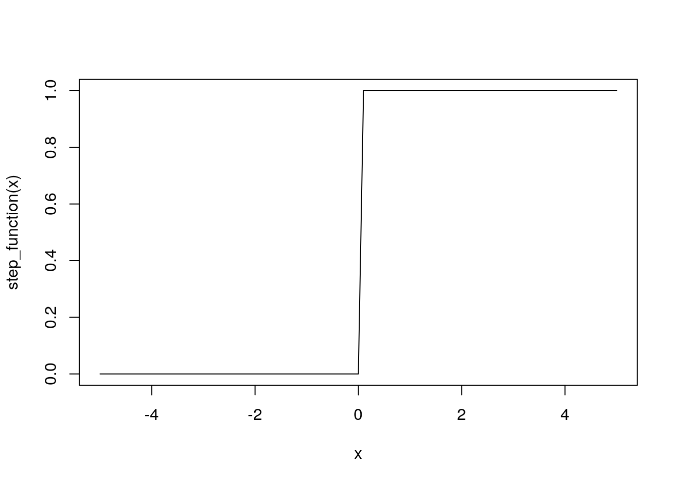

シグモイド関数の実装

sigmoid <- function(x) 1 / (1 + exp(-x))

sigmoid(c(-1.0, 1.0, 2.0))

[1] 0.2689414 0.7310586 0.8807971

curve(sigmoid, -5, 5)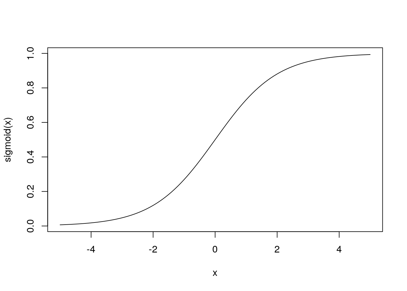

ReLU関数

relu <- function(x) ifelse(x > 0, x, 0)

relu(c(-1.0, 1.0, 2.0))

[1] 0 1 2

curve(relu, -5, 5)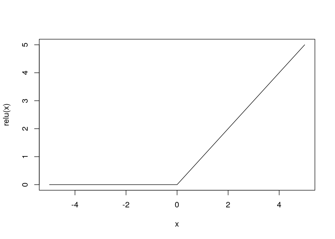

出力層の設計

ソフトマックス関数の実装

softmax <- function(a) {
  exp_a <- exp(a)
  exp_a / sum(exp_a)
}

softmax(c(0.3, 2.9, 4.0))

[1] 0.01821127 0.24519181 0.73659691

オーバーフローに関する問題

softmax(c(1010, 1000, 990))

[1] NaN NaN NaN

対策

softmax <- function(a) {
  exp_a <- exp(a - max(a))
  exp_a / sum(exp_a)
}

softmax(c(1010, 1000, 990))

[1] 9.999546e-01 4.539787e-05 2.061060e-09

手書き数字認識

MNISTデータセットのダウンロード、読み込みにdslabsパッケージを使う。

ディレクトリmnist_dirにデータをダウンロードすることにする。

mnist_dir <- "input/mnist/"
file.exists(mnist_dir)

[1] TRUE

データをダウンロードして読み込む。

mnist <- dslabs::read_mnist(download = TRUE, destdir = mnist_dir)

一度ダウンロードすれば、以降はダウンロードしたディレクトリからデータを読み込める。

mnist <- dslabs::read_mnist(path = mnist_dir)

データ構造を確認

str(mnist)

List of 2
 $ train:List of 2
  ..$ images: int [1:60000, 1:784] 0 0 0 0 0 0 0 0 0 0 ...
  ..$ labels: int [1:60000] 5 0 4 1 9 2 1 3 1 4 ...
 $ test :List of 2
  ..$ images: int [1:10000, 1:784] 0 0 0 0 0 0 0 0 0 0 ...
  ..$ labels: int [1:10000] 7 2 1 0 4 1 4 9 5 9 ...

MNIST画像を表示してみる。

img_show <- function(img) {
  image(matrix(img, nrow = 28)[, 28:1], col = gray(1:12 / 12))
}

ラベルを確認

mnist$train$labels[1]

[1] 5

画像を表示

img_show(mnist$train$images[1, ])

学習済みのパラメータ、sample_weight.pklをダウンロード

url <- "https://github.com/oreilly-japan/deep-learning-from-scratch/raw/master/ch03/sample_weight.pkl"
download.file(url, "input/sample_weight.pkl")

reticulateパッケージのpy_load_object関数を使ってpickleファイルを読み込む。

network <- reticulate::py_load_object("input/sample_weight.pkl")

中身を確認

str(network)

List of 6
 $ b2: num [1:100(1d)] -0.01471 -0.07215 -0.00156 0.122 0.11603 ...
 $ W1: num [1:784, 1:50] -0.00741 -0.0103 -0.01309 -0.01001 0.02207 ...
 $ b1: num [1:50(1d)] -0.0675 0.0696 -0.0273 0.0226 -0.22 ...
 $ W2: num [1:50, 1:100] -0.1069 0.2991 0.0658 0.0939 0.048 ...
 $ W3: num [1:100, 1:10] -0.422 -0.524 0.683 0.155 0.505 ...
 $ b3: num [1:10(1d)] -0.06024 0.00933 -0.0136 0.02167 0.01074 ...

推論処理を行うニューラルネットワークの実装

rep_row <- function(x, n) matrix(rep(x, n), n, byrow = TRUE)

predict <- function(network, x) {
  n <- nrow(x)
  if (is.null(n)) n <- 1

  a1 <- x %*% network$W1 + rep_row(network$b1, n)
  z1 <- sigmoid(a1)
  a2 <- z1 %*% network$W2 + rep_row(network$b2, n)
  z2 <- sigmoid(a2)
  a3 <- z2 %*% network$W3 + rep_row(network$b3, n)

  softmax(a3)
}

推論を実行

library(tidyverse)

# 正規化
images <- mnist$test$images / 255

preds <- 1:nrow(images) %>%
  map(~ predict(network, images[., ])) %>%
  map_int(which.max) - 1

head(preds)

[1] 7 2 1 0 4 1

認識精度

accuracy <- mean(preds == mnist$test$labels)
accuracy

[1] 0.9352

誤認識した画像を確認

misrecognitions <- tibble(actual = mnist$test$labels, pred = preds) %>%
  mutate(i = row_number(), .before = 1) %>%
  filter(actual != pred)

misrecognitions %>% head(12)

# A tibble: 12 × 3
       i actual  pred
   <int>  <int> <dbl>
 1     9      5     6
 2    34      4     6
 3    67      6     2
 4    93      9     4
 5   125      7     4
 6   150      2     9
 7   218      6     5
 8   234      8     7
 9   242      9     8
10   246      3     5
11   248      4     2
12   260      6     0

par(mfrow = c(3, 4))

misrecognitions %>%
  head(12) %>%
  pull(i) %>%
  walk(~ img_show(mnist$test$images[., ]))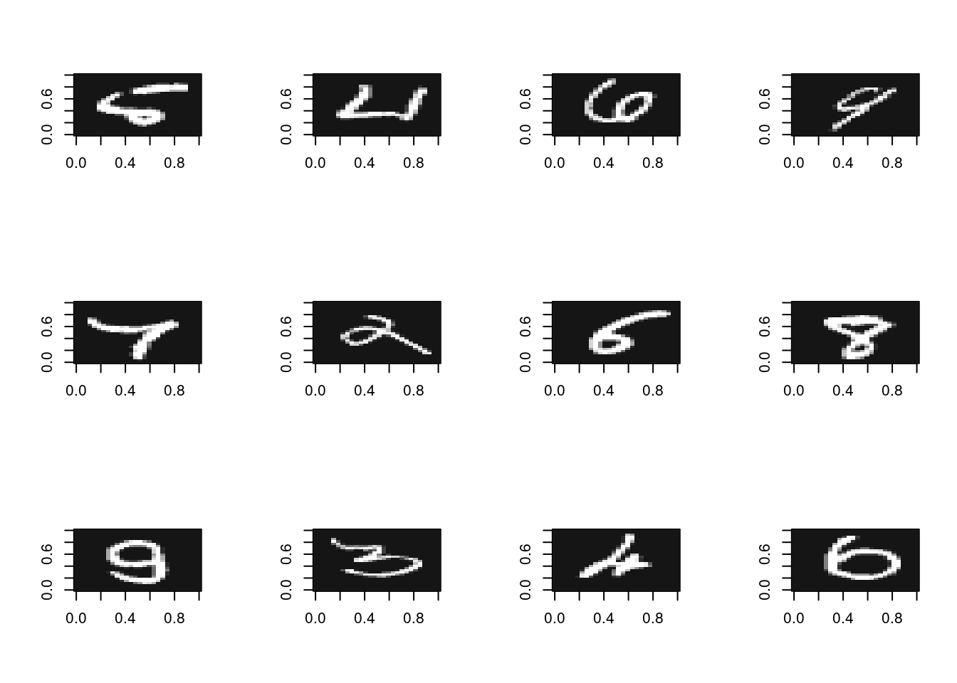

バッチ処理による実行

batch_size <- 100

preds2 <- seq(1, nrow(images), batch_size) %>%
  map(~ predict(network, images[.:(. + batch_size - 1), ])) %>%
  reduce(rbind) %>%
  apply(1, which.max) - 1

identical(preds, preds2)

[1] TRUE