4章 ニューラルネットワークの学習

準備

library(tidyverse)
library(R6)

source("common/functions.R")

損失関数

交差エントロピー誤差

cross_entropy_error <- function(y, t) {
  if (is.vector(y)) {
    y <- matrix(y, 1)
    t <- matrix(t, 1)
  }

  if (identical(dim(t), dim(y))) {
    t <- apply(t, 1, which.max) - 1
  }

  batch_size <- nrow(y)

  -sum(log(map2_dbl(1:batch_size, t, ~ y[.x, .y + 1]) + 1e-7)) / batch_size
}

y  <- c(0.1, 0.05, 0.6, 0.0, 0.05, 0.1, 0.0, 0.1, 0.0, 0.0)

one-hot表現

t <- c(0, 0, 1, 0, 0, 0, 0, 0, 0, 0)
cross_entropy_error(y, t)

[1] 0.5108255

ラベル

cross_entropy_error(y, 2)

[1] 0.5108255

バッチデータ

y2 <- matrix(seq(0.1, 0.6, 0.1), 2, byrow = TRUE)
t2 <- matrix(c(0, 1, 0, 0, 0, 1), 2, byrow = TRUE)
cross_entropy_error(y2, t2)

[1] 1.060131

cross_entropy_error(y2, c(1, 2))

[1] 1.060131

勾配

勾配

numerical_gradient <- function(f, x) {
  h <- 1e-4
  if (is.vector(x)) x <- matrix(x, 1)
  grad <- matrix(0, nrow(x), ncol(x))

  for (i in 1:nrow(x)) {
    for (j in 1:ncol(x)) {
      x1 <- identity(x)
      x1[i, j] <- x[i, j] + h
      x2 <- identity(x)
      x2[i, j] <- x[i, j] - h
      grad[i, j] <- (f(x1) - f(x2)) / (2 * h)
    }
  }

  grad
}

function_2 <- function(x) sum(x ^ 2)

numerical_gradient(function_2, c(3.0, 4.0))

     [,1] [,2]
[1,]    6    8

numerical_gradient(function_2, c(0.0, 2.0))

     [,1] [,2]
[1,]    0    4

numerical_gradient(function_2, c(3.0, 0.0))

     [,1] [,2]
[1,]    6    0

勾配法

勾配降下法

gradient_descent <- function(f, init_x, lr = 0.01, step_num = 100) {
  x <- init_x
  for (i in 1:step_num) {
    x <- x - lr * numerical_gradient(f, x)
  }
  x
}

もしくは

gradient_descent <- function(f, init_x, lr = 0.01, step_num = 100) {
  reduce(1:step_num, ~ .x - lr * numerical_gradient(f, .x), .init = init_x)
}

init_x <- c(-3.0, 4.0)
gradient_descent(function_2, init_x, lr = 0.1, step_num = 100)

              [,1]         [,2]
[1,] -6.111108e-10 8.148144e-10

勾配法による更新のプロセス

gradient_descent_history <- function(f, init_x, lr = 0.01, step_num = 100) {
  accumulate(1:step_num, ~ .x - lr * numerical_gradient(f, .x), .init = init_x)
}

x_history <- gradient_descent_history(function_2, matrix(init_x, 1), lr = 0.1, step_num = 20)
x_history_df <- x_history %>%
  reduce(rbind) %>%
  as.data.frame %>%
  set_names("x0", "x1")

head(x_history_df)

        x0      x1
1 -3.00000 4.00000
2 -2.40000 3.20000
3 -1.92000 2.56000
4 -1.53600 2.04800
5 -1.22880 1.63840
6 -0.98304 1.31072

plot(x_history_df)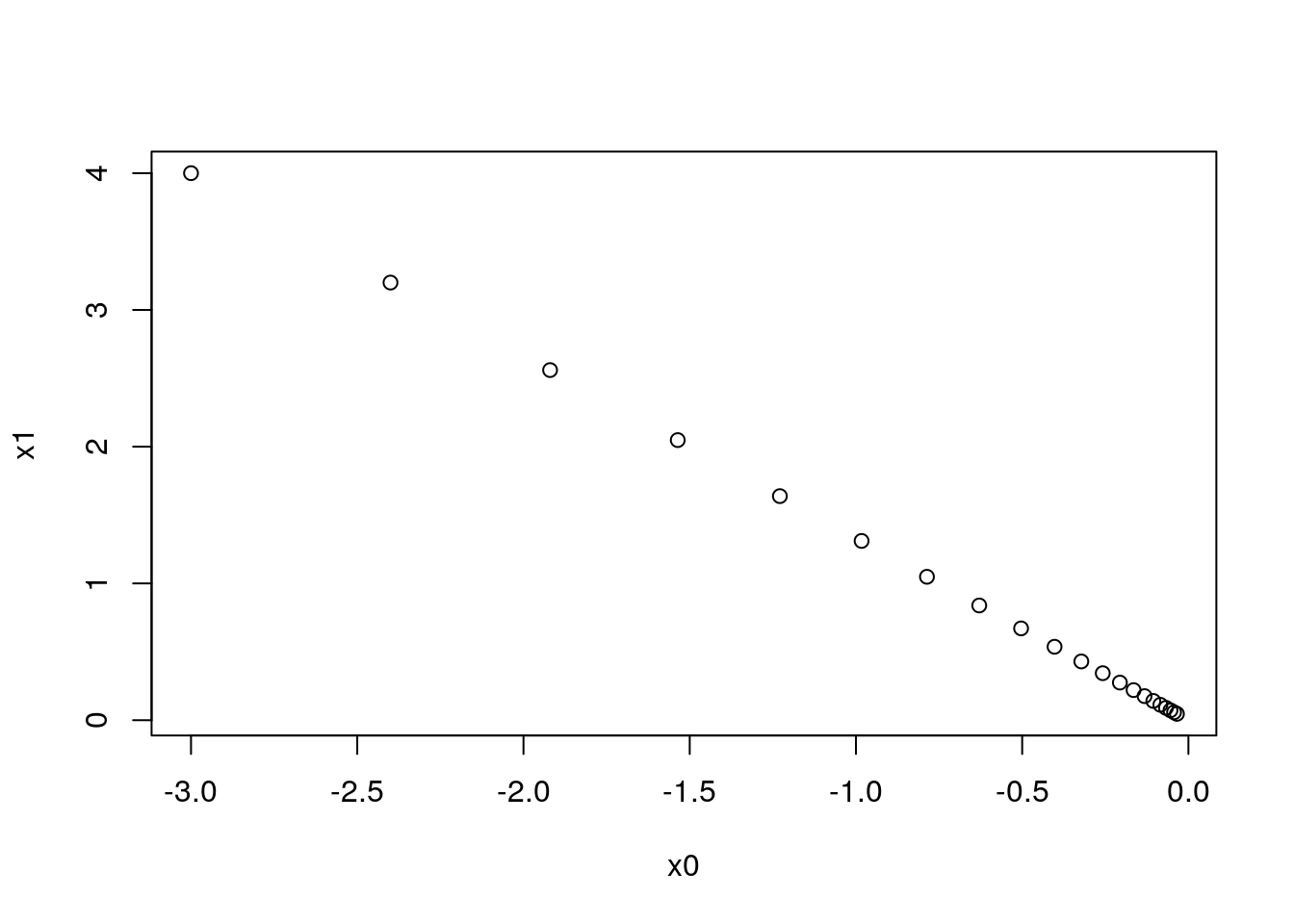

ニューラルネットワークに対する勾配

SimpleNet <- R6Class("SimpleNet", list(
  W = NULL,
  initialize = function(W) self$W <- W,
  predict = function(x) x %*% self$W,
  loss = function(x, t) {
    z <- self$predict(x)
    y <- softmax(z)
    cross_entropy_error(y, t)
  },
  loss_function = function(x, t) {
    w_orig <- self$W
    function(w) {
      self$W <- w
      loss <- self$loss(x, t)
      self$W <- w_orig
      loss
    }
  }))

W <- matrix(c(0.47355232, 0.9977393, 0.84668094,
              0.85557411, 0.03563661, 0.69422093),
            2, byrow = TRUE)
net <- SimpleNet$new(W)
x <- c(0.6, 0.9)
p <- net$predict(x)
p

         [,1]      [,2]     [,3]
[1,] 1.054148 0.6307165 1.132807

t <- matrix(c(0, 0, 1), 1)
net$loss(x, t)

[1] 0.9280683

勾配

f <- net$loss_function(x, t)
numerical_gradient(f, net$W)

          [,1]      [,2]      [,3]
[1,] 0.2192476 0.1435624 -0.362810
[2,] 0.3288714 0.2153436 -0.544215

fは重みを受け取って損失を返す関数。

学習アルゴリズムの実装

2層ニューラルネットワークのクラス

TwoLayerNet <- R6Class("TwoLayerNet", list(
  params = NULL,
  initialize = function(input_size, hidden_size, output_size,
                        weight_init_std = 0.01) {
    self$params <- list()
    self$params$W1 <- matrix(rnorm(input_size * hidden_size, sd = weight_init_std),
                             input_size, hidden_size)
    self$params$b1 <- matrix(0, ncol = hidden_size)
    self$params$W2 <- matrix(rnorm(hidden_size * output_size, sd = weight_init_std),
                             hidden_size, output_size)
    self$params$b2 <- matrix(0, ncol = output_size)
  },
  predict = function(x) {
    n <- nrow(x)
    if (is.null(n)) n <- 1

    a1 <- x %*% self$params$W1 + rep_row(self$params$b1, n)
    z1 <- sigmoid(a1)
    a2 <- z1 %*% self$params$W2 + rep_row(self$params$b2, n)

    softmax(a2)
  },
  loss = function(x, t) {
    y <- self$predict(x)
    cross_entropy_error(y, t)
  },
  loss_function = function(name, x, t) {
    w_orig <- self$params[[name]]
    function(w) {
      self$params[[name]] <- w
      loss <- self$loss(x, t)
      self$params[[name]] <- w_orig
      loss
    }
  },
  numerical_gradient = function(x, t) {
    list(
      W1 = numerical_gradient(self$loss_function("W1", x, t), self$params$W1),
      b1 = numerical_gradient(self$loss_function("b1", x, t), self$params$b1),
      W2 = numerical_gradient(self$loss_function("W2", x, t), self$params$W2),
      b2 = numerical_gradient(self$loss_function("b2", x, t), self$params$b2)
    )
  }))

net <- TwoLayerNet$new(input_size = 784, hidden_size = 100, output_size = 10)
net$params %>% map(dim)

$W1
[1] 784 100

$b1
[1]   1 100

$W2
[1] 100  10

$b2
[1]  1 10

ダミーの入力データと正解ラベル

x <- matrix(runif(100 * 784), 100)
t <- matrix(runif(100 * 10), 100)

勾配を計算

grads <- net$numerical_gradient(x, t)